Lecture 7: Practical Issues in Data Analysis

Initial setup

Multiple testing

Suppose we conduct a randomized study comparing a treatment with a control group.

We have 20 different outcomes and a separate research question for each:

Does treatment affect this outcome?

For each outcome \(j\):

\[\large H_{0j}: \mu_{j1} - \mu_{j0} = 0, \qquad j=1,\ldots,20\]

where \(\mu_{j1}\) and \(\mu_{j0}\) are the population means for outcome \(j\) in the treatment and control groups.

Suppose all 20 null hypotheses are true — treatment has no effect on any of the outcomes.

For any one test with \(\alpha=0.05\), the probability of a Type I error is 5%.

But we are conducting 20 tests.

How likely are we to find at least one statistically significant effect and conclude that the treatment “works”?

Simulating the study

Let’s simulate this study under the assumption that all 20 null hypotheses are true.

For each outcome, we will generate data from the same population distribution for the treatment and control groups:

\[\large Y_{j1},Y_{j0} \sim N(45,3)\]

We will then test for a treatment effect separately for each of the 20 outcomes.

One simulated study doesn’t tell us how often this happens. What if we repeat the entire study many times?

Let’s repeat the study many times . . .

In every simulated study:

all 20 null hypotheses are true
we test each outcome using \(\alpha=0.05\)
we record how many null hypotheses are rejected

In about 64% of studies, at least one of the 20 tests is statistically significant.
Each individual test still has a 5% Type I error rate.
But across the family of 20 tests, the probability of making at least one Type I error is much larger than 5%.
The probability of making at least one Type I error across the family is called the family-wise error rate (FWER):

\[\large \text{FWER} = P(\text{at least one Type I error})\]

For 20 independent tests, the probability that we make no Type I errors is

\[\large (1-0.05)^{20}=0.95^{20}\approx0.36\]

\[\large P(\text{at least one Type I error}) =1-0.95^{20} \approx0.64.\]

Visualizing the problem

It is easier to see what is happening if we consider a smaller family of 5 outcomes.

The figure shows 100 simulated studies. In each study:

all 5 null hypotheses are true
each vertical line is a 95% confidence interval
a red interval does not include 0 and represents a Type I error
shaded columns identify studies with at least one Type I error

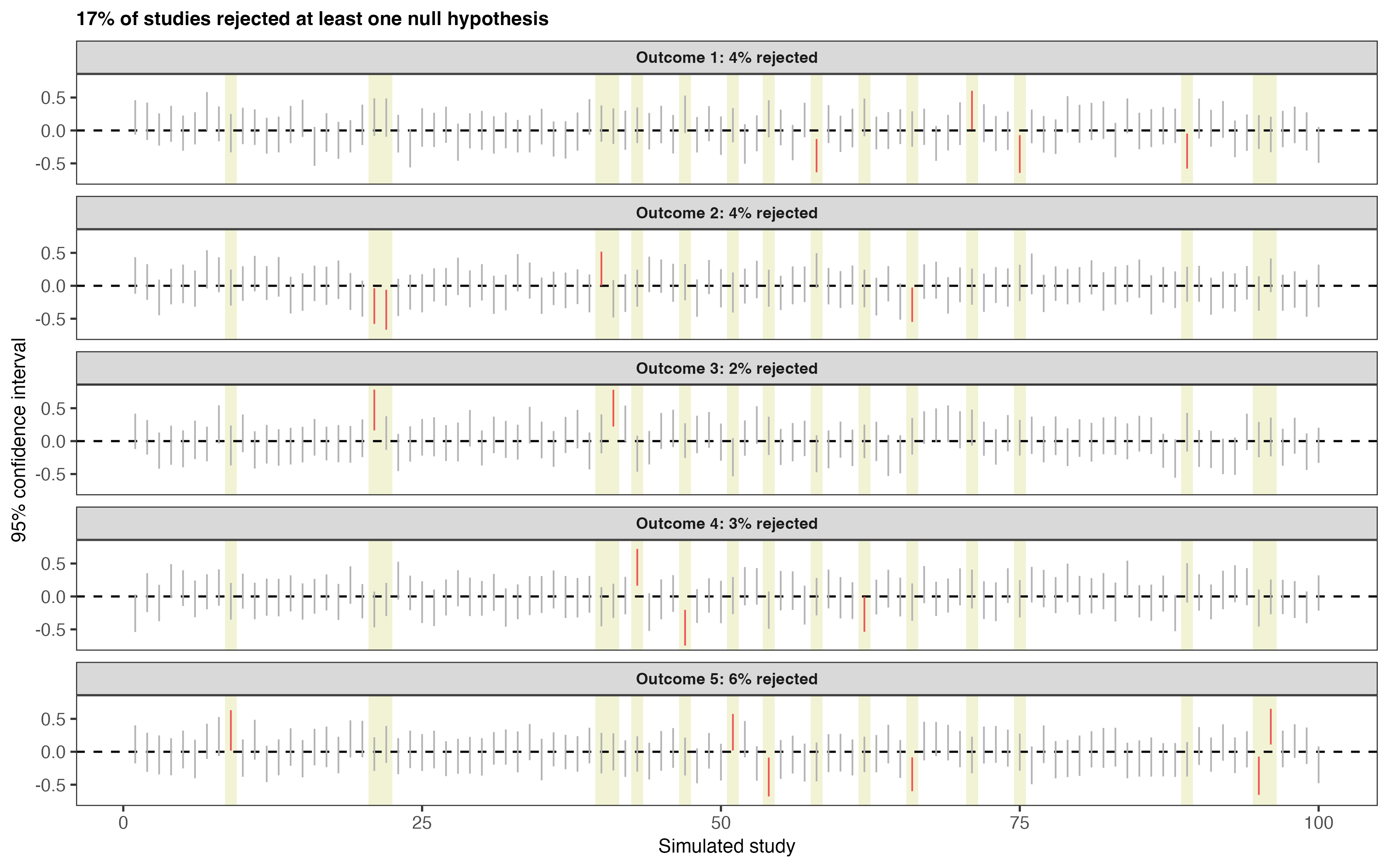
The expected Type 1 error rate with 5 outcomes is:

Controlling the family-wise error rate

We would like the probability of making at least one Type I error across all 20 tests to be no more than 5%.

Can we change the significance level for each individual test so that the FWER is controlled at 5%?

One simple approach is the Bonferroni correction.

Instead of testing each hypothesis using \(\alpha=0.05\), divide \(\alpha\) by the number of tests:

\[\large \alpha^*=\frac{\alpha}{m}\]

where \(m\) is the number of tests.

For our 20 outcomes:

\[\large \alpha^*=\frac{0.05}{20}=0.0025\]

We now reject an individual null hypothesis only when \(p < 0.0025\):

The Bonferroni correction controls the FWER because each individual test now has a Type I error probability of only 0.0025:

\[\large \text{FWER} \leq 20(0.0025) = 0.05\]

The \(\leq\) is important:

Bonferroni guarantees that the FWER is no greater than 5% — it does not have to be exactly 5%.
Unlike \(1-(0.95)^{20}\), Bonferroni does not require the tests to be independent.
This is useful because outcomes in the same study are often correlated.

But there is a tradeoff:

By making it harder to reject each null hypothesis, Bonferroni also makes it harder to detect real effects.

The Holm procedure

Suppose we conduct five tests and obtain these ordered p-values:

\[\large 0.003,\quad 0.009,\quad 0.015,\quad 0.031,\quad 0.20\]

With Bonferroni, every p-value is compared with

\[\large \frac{0.05}{5}=0.01.\]

Only the first two null hypotheses would be rejected.

Holm starts with the same threshold, but becomes progressively less stringent:

compare the smallest p-value with \(0.05/5\)
if rejected, compare the next with \(0.05/4\)
continue until a p-value fails to meet its threshold

p-value	Holm threshold	Decision
0.003	\(0.05/5=0.010\)	Reject
0.009	\(0.05/4=0.0125\)	Reject
0.015	\(0.05/3=0.0167\)	Reject
0.031	\(0.05/2=0.025\)	Stop
0.200	—	Do not reject

Once a p-value fails to meet its threshold, the procedure stops.

Here, Bonferroni rejects 2 hypotheses; Holm rejects 3.

Holm controls the FWER just as Bonferroni does, but can have greater power.

Once the p-values have been adjusted, we compare them with the original significance level. In this case:

Reject the null hypothesis if the adjusted p-value is less than 0.05.

When all of the null hypotheses are true, Holm and Bonferroni have the same probability of making at least one rejection. Holm gains power after the first rejection by using progressively less stringent thresholds.

For controlling the FWER, Holm is generally preferred to Bonferroni because it provides the same error control while being at least as powerful.

Connecting back to ANOVA

In ANOVA, we may want to compare all pairs of group means.

With four groups, there are six pairwise comparisons:

\[\large \mu_1-\mu_2,\quad \mu_1-\mu_3,\quad \mu_1-\mu_4,\quad \mu_2-\mu_3,\quad \mu_2-\mu_4,\quad \mu_3-\mu_4\]

These six comparisons form another family of hypothesis tests, so we again need to consider the FWER.

Bonferroni and Holm are general-purpose methods for controlling the FWER.
The Tukey method is designed specifically for the situation in which we want to make all pairwise comparisons among a set of group means.
Rather than treating the comparisons as unrelated tests, Tukey takes advantage of their common structure.
Without going into the details, Tukey uses the studentized range distribution, which essentially asks:

If all the population means were equal, how far apart might the most separated sample means be simply because of sampling variability?

Tukey uses this distribution to choose a critical value for the pairwise differences. This produces wider confidence intervals — and larger adjusted p-values — than we would get by treating each comparison separately, while controlling the FWER.

False discovery rate

So far, we have focused on the family-wise error rate:

FWER: How likely are we to make any false discoveries?

But there is another way to think about errors when we conduct many tests:

FDR: What is the expected proportion of our discoveries that will be false?

Suppose we are testing 10,000 genes to identify genes that may be associated with a disease.

Controlling the FWER means trying to keep the probability of making even one false discovery among the 10,000 tests below 5%.

Using Bonferroni, we would require

\[\large p < \frac{0.05}{10{,}000}=0.000005.\]

That is an extremely stringent threshold — and may be more stringent than we need.

Instead, we might be willing to tolerate some false discoveries, as long as they represent only a small proportion of all the discoveries we make.

False discovery proportion

Among the results we call statistically significant — our discoveries — some may be:

true discoveries — there really is an effect
false discoveries — Type I errors

For a particular study, the false discovery proportion (FDP) is

\[\large \text{FDP} = \frac{\text{number of false discoveries}} {\text{total number of discoveries}}.\]

For example, if 8 of 100 discoveries are false:

\[\large \text{FDP}=\frac{8}{100}=0.08.\]

But FDP describes what happened in one particular study.

The false discovery rate (FDR) is the expected FDP across repeated studies:

\[\large \text{FDR}=E(\text{FDP}).\]

This gives us two different ways of controlling errors across repeated studies:

FWER: How likely are we to make any false discoveries?
FDR: What is the expected proportion of our discoveries that will be false?

Controlling the FDR at 5% does not mean that exactly 5% of the discoveries in every study will be false.

Would the false discovery proportion always be about 39%?

Repeating the study

Now let’s repeat the entire study many times.

For each simulated study, we calculate the false discovery proportion.

The false discovery rate is the expected FDP across repeated studies:

\[\large \text{FDR}=E(\text{FDP})\]

Controlling the false discovery rate

Can we control the proportion of our discoveries that are false without being as stringent as controlling the probability of even one false discovery?

The Benjamini-Hochberg (BH) procedure is designed to do just that.

Let’s first see what it does before looking at how it works.

The FDP describes this particular study. What happens if we repeat the study many times?

Across repeated studies, the average FDP — the false discovery rate — is approximately 5%.

The Benjamini-Hochberg procedure

The Benjamini-Hochberg (BH) procedure controls the false discovery rate.

Like Holm, BH begins by ordering the p-values from smallest to largest:

\[\large p_{(1)} \leq p_{(2)} \leq \cdots \leq p_{(m)}.\]

Suppose we have five tests and want to control the FDR at 5%.

BH compares each ordered p-value with

\[\large \frac{i}{m}(0.05),\]

where \(i\) is the position of the p-value in the ordered list.

For five tests, the thresholds are:

\(i\)	BH threshold
1	\((1/5)(0.05)=0.01\)
2	\((2/5)(0.05)=0.02\)
3	\((3/5)(0.05)=0.03\)
4	\((4/5)(0.05)=0.04\)
5	\((5/5)(0.05)=0.05\)

BH finds the largest p-value that satisfies its threshold:

\[\large p_{(i)} \leq \frac{i}{m}(0.05).\]

\(i\)	p-value	BH threshold
1	0.008	0.010	✓
2	0.021	0.020
3	0.027	0.030	✓
4	0.046	0.040
5	0.200	0.050

The largest p-value satisfying the criterion is \(p_{(3)}=0.027\), so BH rejects the first three null hypotheses.

Unlike Holm, BH does not stop when an individual p-value fails its threshold.

The idea behind the increasing thresholds is that BH permits a larger p-value cutoff because FDR allows some false discoveries when there are more discoveries overall.

Here, BH supports three discoveries, so the cutoff is

\[\large \frac{3}{5}(0.05)=0.03.\]

All three smallest p-values are below 0.03, so all three null hypotheses are rejected.

More generally, BH searches for the largest set of discoveries that satisfies the FDR criterion.

Unlike FWER control, the goal is not to avoid every false discovery — it is to control the expected proportion of discoveries that are false.

Missing data

Suppose we want to estimate the average outcome in a population.

Our research question is:

What is the population mean outcome?

Ideally, we would observe all of the variables we planned to collect for every participant.

But in real studies, some data are often missing:

some participants may be missing the outcome
others may be missing baseline characteristics or other covariates

When does missing data create a problem for our analysis?

Starting with missing outcomes

Let’s start with a simple sampling process in which the outcome is missing for some participants.

We will simulate 1,000 participants:

a baseline health score \(X\), observed for everyone
mean outcome of 50 for a participant with \(X=0\)
outcome standard deviation of 10

The baseline health score is related to the outcome:

\[\large X_i \sim N(0,1)\]

\[\large Y_i = 50 + 5X_i + \epsilon_i, \qquad \epsilon_i \sim N(0,10)\]

Because we are simulating the data, we know the true population mean is 50.

The gray line shows the true population mean of 50; the dashed line shows the mean in our simulated sample.

What if outcomes disappear randomly?

Suppose each participant has a 30% chance of having a missing outcome.

The probability of missingness is unrelated to:

baseline health
the value of the outcome

The dashed line now shows the mean among participants whose outcomes are observed.

Repeating the study

Now let’s repeat the sampling many times.

In each simulated study, we estimate the population mean using:

the complete data
the observed data after 30% of outcomes are missing

On average, both analyses recover the true population mean of 50.

But the estimates based on the incomplete data vary more from study to study:

Randomly losing outcomes costs us information and precision, but does not systematically shift the estimate of the population mean.

This type of missingness is called Missing Completely at Random (MCAR):

The probability that a value is missing does not depend on any observed or unobserved data.

What if missingness depends on something we observed?

Now suppose the probability that the outcome is missing depends on the participant’s baseline health score.

Participants with lower baseline health scores are more likely to have a missing outcome.

Because baseline health is observed for everyone, we know something about why the outcome is missing.

Repeating the study

Because baseline health predicts the outcome, systematically losing participants with lower health scores may also change the mean outcome among those we observe.

When missingness depends on an observed variable that is related to the outcome, simply analyzing the observed outcomes can produce a biased estimate of the population mean.

This type of missingness is called Missing at Random (MAR):

The probability that a value is missing may depend on observed data, but — after accounting for those observed data — does not depend on the missing value itself.

Using the information we observed

Under MAR, we have information that helps explain why some outcomes are missing.

In our example:

baseline health is observed for everyone
baseline health predicts the outcome
baseline health also predicts whether the outcome is missing

Can we use baseline health to recover the population mean?

First, we estimate the relationship between baseline health and the outcome using participants whose outcomes were observed:

We can then use this model to predict the outcome for everyone in our sample based on their observed baseline health:

Instead of averaging only over the selected group with observed outcomes, we used information from the full sample to estimate the population mean.

This is one example of a model-based approach to handling missing data under MAR.

Multiple imputation

Another common approach for handling missing data under MAR is multiple imputation.

Multiple imputation uses the observed data to create several plausible completed datasets, rather than treating any single prediction for a missing value as if it were known.

Each completed dataset is analyzed separately, and the results are then combined.

Because the missing values differ across the completed datasets, the final analysis reflects uncertainty about the data we did not observe.

Multiple imputation does not recover the missing values — it represents plausible values and our uncertainty about them using the information we did observe.

What if missingness depends on what we did not observe?

Now suppose the probability that an outcome is missing depends on the value of the outcome itself.

Participants with lower outcome values are more likely to have a missing outcome.

Here, participants with lower outcomes are systematically more likely to be missing, inflating our estimate of the population mean.

But there is an important difference from our previous example:

For participants whose outcomes are missing, we do not observe the information that explains why they are missing.

Repeating the study

Let’s again repeat the sampling process many times.

When the probability of missingness depends on the missing outcome itself, the observed outcomes may systematically differ from the outcomes we did not observe.

This type of missingness is called Missing Not at Random (MNAR):

Even after accounting for the observed data, the probability that a value is missing depends on the value that is missing.

Can we tell whether data are MNAR?

Usually, we cannot determine from the observed data whether missingness is MAR or MNAR.

For participants with missing outcomes, we do not know what those outcomes would have been. Therefore, we cannot directly determine whether missingness depends on those unobserved values.

However, an MAR assumption may be more reasonable when we have good observed information about:

factors that predict whether data are missing
factors that predict the missing outcome

For example, if participants in poorer health are more likely to have missing outcomes, detailed measures of their health before the outcome is missing may help make an MAR assumption more plausible.

We cannot prove that data are MAR, but collecting and using variables that help explain both the outcome and missingness can make the assumption more reasonable.

Can observed information solve the problem?

We can try the same model-based approach we used under MAR:

Under MNAR, observed variables may help, but they cannot fully account for missingness that still depends on the unobserved value itself.

What can we do about MNAR?

Because we cannot know the missing outcomes, there is no purely data-driven solution to MNAR.

Instead, we can conduct sensitivity analyses:

Make different assumptions about the missing outcomes and ask whether our conclusions change.

More formal statistical methods for MNAR follow the same basic principle: they require assumptions about the data we did not observe.

Missing data: putting it together

MCAR: Missingness does not depend on observed or unobserved data.
- Analyzing the observed data may cost precision; in our example, it does not systematically shift the estimate.
MAR: Missingness can depend on information we observed.
- We can use that observed information to help account for the missing data.
MNAR: Missingness still depends on information we did not observe.
- Observed information may help, but additional assumptions are needed to account fully for the missing data.

The consequences of missing data depend on why the data are missing — not simply on how much data are missing.